Algorithm to find the Chinese horoscope sign of any year

After learning about modulo function, I finally have an elegant algorithm to find out the Chinese horoscope sign based on the year of input. It came from an innocent enough question from facebook - what's the value of m+n, such that 2012^m and 2012^n has the same last 3 digits, if m and n are integers are m is greater than m?

I did a bit of exploring and found out the answer by doing it through excel. Then I discovered the modulo function, and then I also discovered the theorem that if a = b (mod m), then a^c = b^c (mod m). It's vastly different from learning about mathematical theorem through books or teachers, and learning about it through discovery. The joy of solving the puzzle is immensely satisfying.

But first of all, what's the modulo function?

Modulo function has two inputs i.e. MOD (a, b). Basically the function just returns you the number that is the remainder if a is divided by b. For example, MOD (12, 3) = 0 because 12 divided by 3 gives no remainder. MOD (12, 5) = 2 because 12 divided by 5 gives a remainder of 2.


My algorithm to find out the Chinese astrological sign is to take the input year, subtract 4 to it, modulo it to 12, then add 1 to the result. You can use it on excel.

i.e. Let x be the input year

y = MOD(x-4, 12) + 1

The output y will give you a number ranging from 1 to 12, so

1 is rat,
2 is ox,
3 is tiger,
4 is rabbit,
5 is dragon,
6 is snake,
7 is horse,
8 is goat,
9 is monkey,
10 is rooster,
11 is dog and
12 is pig.

To illustrate this, let's try out the year 3194:

So in the year 3194, y = MOD(3194-4, 12) +1 = 11, so it’s the year of the dog.

Read More

I played 800 games of 100 coin toss

You have to read this article before this to make sense of what I'm saying here.


After putting up the probability distribution and showing that after playing 100 toss of coin, where each head gives you $2 and each tail takes away $1 from you, will not always give you a positive returns, I was still unsatisfied.


I went ahead and did a monte carlo simulation of the game on excel. Using RAND() function, I will get a random value between 0 and 1. I programmed it such that if I have a number bigger or equal to 0.5, it'll be heads and I'll assign a value of 1 to it. If not, it'll be tails and I'll assign a value of 0 to it.

IF( cell >= 0.5, 1, 0) 

After tallying the number of heads and tails, I proceed to count the gain/loss from this 100 toss game. I did 800 simulation of such 100 coin toss, effectively throwing 80,000 coins in my computer program.

HUAT AH!

Here's the results of all 800 such games of 100 coin tosses. The numbers in each cell represents the gain/loss from playing the game:

I highlighted 2 cells in yellow because this is what I get after playing 800 such games - I've two games where I have negative returns! The probability is higher than the initial theoretical calculation. The theoretical probability of ending up having losses after 100 coin tosses is 0.043686%. Based on this monte carlo simulation, I have 2/800 or 0.25% of ending up not being profitable.


I calculated the average score of all these 800 games of 100 coin tosses, and it turns out to be $49.43875, which is very close to the expected value calculated of $50. Just for interest sake, the mode (the sum that occurred most often) of all 800 such games is $53 and the median is $50.


There! The statement that after 100 coin tosses, you always end up being profitable is not true. Combining the new found skills in excel simulation with real life examples is really really interesting LOL

Read More

How to do a 2 variable data table

I was going to teach a student business analytics, which is something I've never really done before. So far so good, it's half statistics, which I already knew but more application type of questions (instead of theoretical ones) somewhat related to making sound business decisions. The other half is about simulation and modelling using mainly excel. I've always wanted to learn the deeper end of excel but never really got the motivation to see down and try out all the fancy stuff. It's not just about learning it, but also applying it to my daily life and see how I can hack out some more productivity out of the things that I do. That's more important for me.


I'm at best a novice user of excel. The formula part of the excel is not a problem for me. It's the more intricate data crunching part that eludes me. So if you're already an excel expert, don't laugh at my feeble attempt.


I happened upon this question where they set up a 2 variable data table to see how it varies the final output. Fancy stuff, didn't even know I could do that! So here's me sharing how to do 2-variable data table, step by step.


So here's my problem: I want to get a sum of money in 30 yrs time. I want to find out how much I can get by using this formula:

Future value (FV) = Present value (PV) x (1 + Rate/100)^time

There are two input variables in here, namely PV and R, and one input constant, which is time. My output data will be FV. Time is fixed at 30 yrs, and the two input variables are rate (of investment returns, at %/pa) and PV (which is the amount that I'm going to invest right now). I want to see how the two variables will affect the output, which is the future value FV, given this particular set of constraints.


I limit my PV to go between $5k and $100k inclusive, and my rate between 0.5% and 8% inclusive.


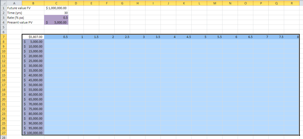
Step 1: Key in the data in excel.

The cell B7 is using the formula: = C4*POWER((1+C3/100),C2). It doesn't matter what rate or PV you used initially. I used 0.5 and $5000 at first, but it doesn't really matter.


Step 2: Key in the rows and columns.

The rows I let it be the rate, ranging from 0.5 to 8 with incremental steps of 0.5%. The columns I let it be the PV starting from 5k to 100k, with incremental steps of 5k. Do note that the rows and columns must be to the right and bottom of the cell B7.

Step 3: Highlight cell B7:R27, as shown below

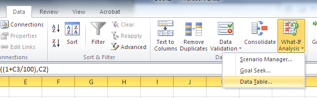
Step 4: Go to Data / What-if-analysis / Data Table and click on it.

Select row input cell as C3 and column input cell as C4. Basically you're telling them that you want the row of cells (C7:R7) to the right of B7 as the Rate (C3) and the columns of cells below B7 (B8:B27) as the PV (C4).


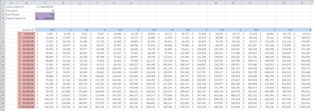
Step 5: Done!

You can now analyse the data based on the different inputs of rate and PV. For example, if you want to reach 200k at the end of 30 yrs, you can do a few options:

1. Put in 20k and invest at 8%
2. Put in 35k and invest at 6%
3. Put in 80k and invest at 3% and many other options


This is seriously going to be helpful for me!

Read More